Scaling Laws for LLM-Based Data Compression
Introduction
The scaling laws for neural language models showed that cross-entropy loss follows a power law in three factors:
- Dataset size
- Model parameters
- Training compute (steps or epochs)
The lower the cross-entropy loss, the better the model’s next-token prediction. Since prediction and compression are deeply linked (The Intricate Link Between Compression and Prediction), a lower loss should translate into better lossless compression. This raises the question:
Do LLMs exhibit clean power-law scaling in compression performance?
Experiment
For the experiment, I considered the Pythia models, which are available at multiple checkpoints and parameter sizes. All Pythia models are trained on the same dataset (The Pile), ensuring a uniform comparison. Following Delétang et al. (2023), The LLM’s predicted probabilities for each token are used to update the symbol table of an arithmetic encoder (a near-optimal entropy coder). I took the first 2048 chunks of the enwik8 dataset each chunk is 2048 bytes and fed them to the LLM to predict the next-token probabilities.
The other experimental parameters are:
- Models: EleutherAI Pythia family (8-bit quantized): 70 M, 160 M, 410 M, 1 B, 1.4 B parameters
- Checkpoints: 1 k, 8 k, 32 k, 128 k, 143 k training steps
- Chunking:
- CHUNK_SIZE: 2048 bytes
- NUM_CHUNKS: 2048 per dataset
- Compression pipeline:
- Raw bytes → ASCII
- Tokenize and pass the ASCII symbols to LLM
- Arithmetic coding on LLM probabilities
- CR = compressed_bits / original_bits
- Datasets & Preprocessing:
- Text: enwik8 (Wikipedia XML)
- Image: ImageNet-1k validation → 32 × 64 grayscale patches (uint8 bytes)
- Speech: LibriSpeech “clean” train.100 → 16 kHz PCM → int16 bytes
Results: Text Compression
| Model | 1 k | 8 k | 32 k | 128 k | 143 k |
|---|---|---|---|---|---|
| pythia-70M | 0.223 | 0.176 | 0.17 | 0.173 | 0.175 |
| pythia-160M | 0.218 | 0.159 | 0.149 | 0.149 | 0.150 |
| pythia-410M | 0.223 | 0.148 | 0.136 | 0.129 | 0.128 |
| pythia-1B | 0.207 | 0.140 | 0.128 | 0.120 | 0.120 |
| pythia-1.4B | 0.207 | 0.137 | 0.124 | 0.115 | 0.115 |
Text scaling-law fit
We fit a Kaplan-style power law
\(\mathrm{CR}(P,S)
= a + b\,P^{-\alpha} + c\,S^{-\beta}.\)
For text, the best-fit coefficients are:
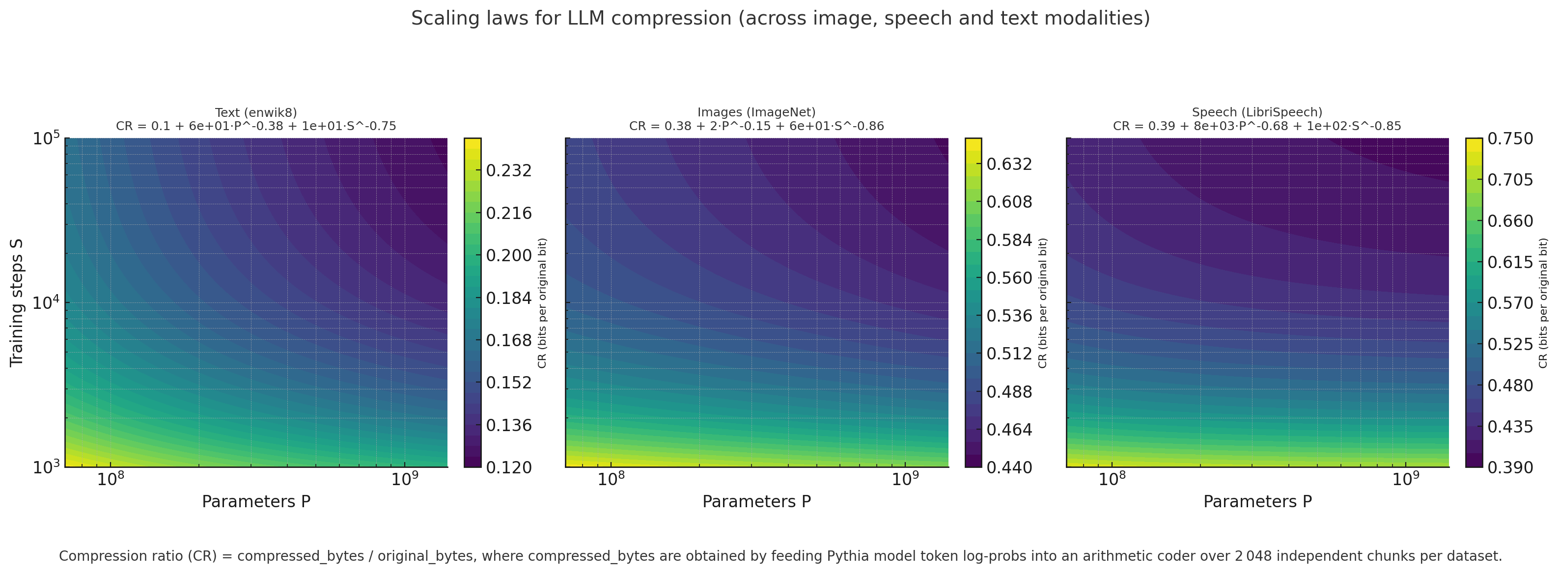
\(\mathrm{CR}_{\text{text}}
= 0.10 + 60\,P^{-0.38} + 10\,S^{-0.75}.\)
Compression on Non-Text Modalities
The “Language Modeling Is Compression” paper shows that an LLM trained only on text can compress arbitrary byte streams Language Modeling Is Compression. I applied the same pipeline to ImageNet-1k patches and LibriSpeech audio.
Image Results
| Model | 1 k | 8 k | 32 k | 128 k | 143 k |
|---|---|---|---|---|---|
| pythia-70M | 0.601 | 0.499 | 0.492 | 0.505 | 0.513 |
| pythia-160M | 0.615 | 0.483 | 0.471 | 0.482 | 0.492 |
| pythia-410M | 0.668 | 0.506 | 0.461 | 0.444 | 0.447 |
| pythia-1B | 0.601 | 0.470 | 0.456 | 0.436 | 0.440 |
| pythia-1.4B | 0.643 | 0.482 | 0.470 | 0.434 | 0.436 |
Image scaling-law fit
\[\mathrm{CR}_{\text{image}} = 0.38 + 2\,P^{-0.15} + 60\,S^{-0.86}.\]Speech Results
| Model | 1 k | 8 k | 32 k | 128 k | 143 k |
|---|---|---|---|---|---|
| pythia-70M | 0.695 | 0.460 | 0.439 | 0.475 | 0.466 |
| pythia-160M | 0.678 | 0.440 | 0.430 | 0.433 | 0.456 |
| pythia-410M | 0.770 | 0.505 | 0.404 | 0.383 | 0.391 |
| pythia-1B | 0.677 | 0.424 | 0.444 | 0.376 | 0.384 |
| pythia-1.4B | 0.752 | 0.469 | 0.443 | 0.378 | 0.385 |
Speech scaling-law fit
\[\mathrm{CR}_{\text{speech}} = 0.39 + 8\times10^{3}\,P^{-0.68} + 1\times10^{2}\,S^{-0.85}.\]Combined Scaling Curves
The below plot shows the overall scaling laws plots across all the three modalities, While the scaling law trend is present in non-textual modalities, the compression is not as strong in text.
Conclusion
It has been argued that LLMs trained only on text can form world models for proto-AGI. These compression results reinforce that claim: despite text-only pretraining, LLMs compress images and speech following clear power laws.
We hypothesize two primary mechanisms responsible for this:
-
In-Context Learning
Within a given token window, self-attention adapts on-the-fly to file-specific patterns (repeating pixels, periodic audio cycles), shaving off most of the entropy. -
Universal Sequence Prior
Pretraining internalizes bursty repetitions, Zipf’s law, heavy tails, and long-range autocorrelations statistics shared by all byte streams. Even without context, compression ratio should be far below uniform-noise rates. Do read Benford’s Law, Zipf’s Law and the Pareto Distribution to know more about naturally occuring data distributions and their universality
A really interesting future work should be to quantify each component’s contribution and trace how they emerge during pretraining.
References
- Kaplan, J.; McCandlish, S.; Henighan, T.; Brown, T.; Chess, B.; Child, R.; Gray, S.; Radford, A.; Wu, J.; Amodei, D. “Scaling Laws for Neural Language Models.” arXiv 2001.08361 (2020). https://arxiv.org/abs/2001.08361
- The Intricate Link Between Compression and Prediction. Mindful Modeler Substack (2024). https://mindfulmodeler.substack.com/p/the-intricate-link-between-compression
- Delétang, G.; Ruoss, A.; Duquenne, P.-A.; Catt, E.; Genewein, T.; Mattern, C.; Grau-Moya, J.; Wenliang, L.K.; Aitchison, M.; Orseau, L.; Hutter, M.; Veness, J. “Language Modeling Is Compression.” arXiv 2309.10668 (2023). https://arxiv.org/abs/2309.10668
- Gao, Leo. “Thoughts on the Alignment Implications of Scaling Language Models.” BMK.sh Blog (2021). https://bmk.sh/2021/06/02/Thoughts-on-the-Alignment-Implications-of-Scaling-Language-Models/
- Tao, T. “Benford’s Law, Zipf’s Law and the Pareto Distribution.” Terence Tao’s Blog (2009). https://terrytao.wordpress.com/2009/07/03/benfords-law-zipfs-law-and-the-pareto-distribution/